Notes on Statistical Learning Theory
Background
Acknowledgement
Much of the content here is drawn from Warwick University's Mathematics of Machine Learning lecture course (2023-24), taught by Clarice Poon. These lecture notes are not publicly available. I'd like to thank Clarice for inspiring this post based on her teaching. Please see the references section for my best efforts at proper attribution. I'll branch off into more original territory in the future!
Personal Context
This post is an experiment. I adored my time studying Clarice Poon's Mathematics of ML during my final year at Warwick (23-24). As I wrestled with the material - like all well taught maths modules - slowly, from the mist, a beautiful story emerged! As a person who thinks in narrative, I've always wondered: what does it look like to actually write down how I understand this kind of technical content? After a year out of formal education working in DESNZ, I wanted my mathematical itch scratched...hence this post.
One of my favourite lecturers said 'mathematics is compressible'. You can take 20 pages of formalism, wrap it up into a single definition, and then when defining some new object, all that complexity can be implicitly assumed! In this post, I've attempted to unwinded that density resulting in a lengthly tract that's frustratingly but inevitably non-self-contained. I'll choose to embrace this meaning the intended audience isn't particularly targeted. To the serious mathematician, I'll be labouring the obvious; to the non-technical, I won't shy away from the symbols.
Regardless, I've enjoyed dipping my toes back into familiar mathematical waters. I hope this post can form a personal benchmark for what it means for me to actually understand a particular topic, giving me something to measure against when I venture off into yet-uncharted territory.
Enough faff - let's get on with it!
Why does Statistical Learning Theory matter?
SLT offers a rigorous mathematical foundation for 'classical' machine learning. While this 30 year old theory isn't exactly cutting-edge and wouldn't be used in practice explicitly, the ideas developed here do form the foundational concepts motivating the current deep-learning paradigm. Besides, purely aesthetically, the mathematical arguments are quite pretty! Hence, I think reminding myself of the foundations of ML before starting a role in Industry will be time well spent.
Of the different types of learning (supervised, unsupervised, reinforcement, etc.), SLT is neatest when describing supervised learning. In this post, I'll further simplify to the case of binary classification (photo of a cat or dog) and build up some theory.
The set-up
Here, our goal is to make a machine learn from labelled categorical data. More precisely, we want to learn a function
A small note that our actual data
The Very Basics
SLT is all about understanding how well our function LINK TO LATER ON
The Hypothesis Class
Firstly, what is this function
As a concrete example,
So here, our hypothesis class
In the real world,
Loss
We now need some way to quantify how well our chosen function LINK TO INTERESTNG NOTE ON LOSS FUNCTIONS
If LINK TO DEEP LEARNING SECTION, the model will keep tweaking its parameters, getting better and better...eventually leading to some pretty stellar ML models.
To assess performance, we need a loss function. This compares the model's predicted label to the real data. If we're correct (or close to correct), then the error (or loss) is low. If our model predicted a label that was far from the original value, then our loss in high.
Formally in our context of binary classification, the loss function
- A real label from data,
, and - A label predicted using our model
and outputs a numerical score telling us how good the guess is.
In our simple context of binary classification, this loss function
Risk
Now we can quantify the performance of our model
We want our model to perform well on all the data,
Formally, in terms of our random variables
Digging into the details of what this expectation actually means, for some fixed hypothesis
The Bayes Classifier
Now we have the goal: find an
In our case of simple binary classification (the only possible labels being
Importantly, there is no restriction on what
The Empirical Risk
None of this has been terribly practical so far. We now turn to the actual data which could be collected in the world (spam emails, cat pictures etc). Say we have
While before, we integrated over the space of all possible values for
From this, again, we ask the question: 'what is the best possible function we can pick to minimise this empirical risk'?
While the Bayes classifier was the best possible function we could ever pick to minimise the total loss, we now restrict to only searching over functions inside our chosen hypothesis class,
This is the empirical risk minimiser, defined to be
This is a far more practical question to answer. We have our chosen hypothesis class
Basic ERM examples
To make this concrete, I'll show how we can find the ERM in some particular examples.
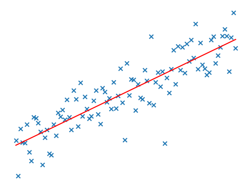
Linear Regression
Classic! Important! For this example, we'll take the case where our feature space
For our loss function, will just take
Well, our empirical risk is simply
It turns out this problem has a neat closed form solution! If we package up our feature vector data
See the annex for the details LINK TO ANNEX - the point is to illustrate how the empirical risk minimiser framework can fit into the framework of classical statistics: finding optimal model parameters based on data. E.g. for
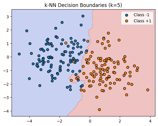
K-Nearest Neighbours
If we return to binary classification, another classic example to demonstrate the practicality of the ERM framework would be k-NN. Here, we have
Say you have training data
And our corresponding hypothesis class are the so called 'Voronoi regions'
Deep Learning
The examples above show how to find the ERM from data for simple
For these more general models, there isn't an explicit analytic solution. Hence, we need to devise an algorithms which can slowly improve the parameters of the model, moving through the space of all possible models,
Formally, for some
- Initialise with
- Iterate using some carefully chosen step size
, sampling iid from
Obviously, there's a lot more to model training than this! The point here is to demonstrate methods which can practically compute an ERM from data in the real world.
Now we have a feel for why finding an ERM is useful and how we can do this in practice, we return to our central question: how do we quantify how well our model is performing? The empirical risk on our current data may be low, but if we then applied this model to unseen data, would it continue to perform as well? How should we go about formalising this difference?
Excess Risk
We've seen what it looks like to pick a model class (e.g. regression, K-NN) and then find the best possible parameters for that model on our data. This is the all important empirical risk minimiser,
We've seen that the Bayes Classifier,
This captures the error in our model class from our 'best case scenario',
It's worth noting that due to various so called 'no free lunch' theorems, without assumptions on our underlying probability distribution, it's impossible to find some empirical risk minimisers which perform arbitrarily well on that data. There's no universal method for learning.
How does this excess risk relate to our all important empirical risk minimiser
The decomposition of excess risk
For our ERM, we picked a chosen hypothesis class
While our empirical risk minimiser found the model in our hypothesis class with the lowest risk on our training data, there could be models in our hypothesis class that have lower overall risk. Formally, we can define this (assuming it exists!) as
Correspondingly, we can use this notion to decompose our excess risk. We want to split these two related, but separate separate ideas:
- First, how well is our ERM
performing inside our chosen model class? We want to quantify the difference between the current performance of our model on our data, and the best this chosen model class can do on all possible data. This is called the estimation error. - Second, how good is our chosen hypothesis class
compared to the best we can ever do over all possible hypothesis classes? This is the approximation error.
Putting these ideas together in the symbols, we have the following formula:
Thinking about what this means in terms of model selection, the larger (and more expressive) you make your hypothesis class
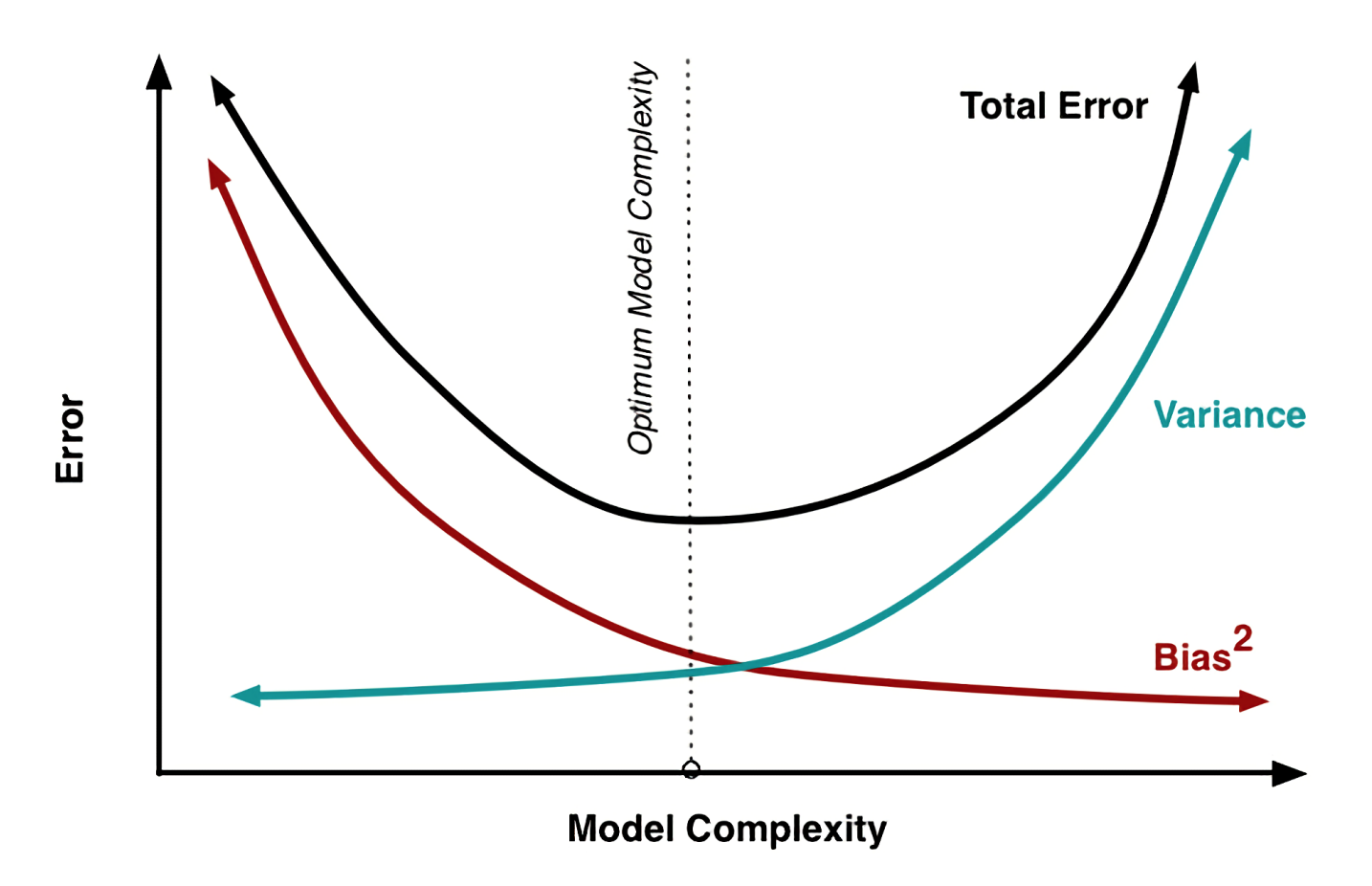
Classic Interpretation
Mapping this onto the classic bias vs variance trade-off graph from statistics, we can say
- Estimation error
Variance: as complexity grows (up to DL-complex), there is more and more space for your ERM trained from data, to diverge from the best possible model within your hypothesis class. - Approximation error
Bias : as model complexity grows, the best model possible within slowly converges towards the best ever possible model, the Bayes Classifier, .
Note on the connection to Deep Learning and modern research
With the advent of deep learning, this classical paradigm has been blown out of the water! By selecting an extremely expressive hypothesis class (transformers etc) and spending huge amounts of computing resource tuning the parameters of the model using vast quantities of data (the entire internet...) companies have been able to find ERMs with near zero excess risk. Blatantly stealing the key image from Belkin, Hsu, Ma, and Mandal's 2019 paper, you can see that with model ML models, the classical graph has a long tail heading right:
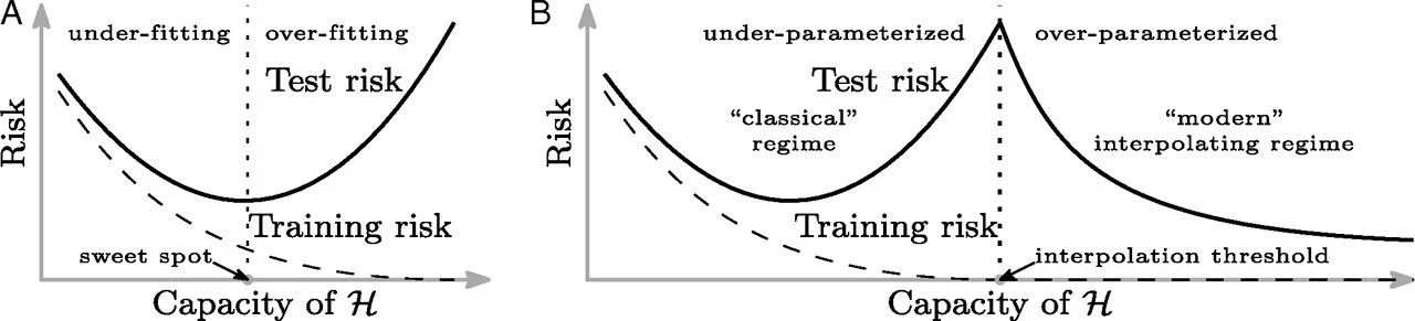
Finally, finding an explanation for this seems to still be an active area of research. Interestingly, in 2022, Sébastien Bubeck and Mark Sellke published a paper which made some theoretical in-roads using some of the tools and techniques that I'll introduce later in this post. LINK TO LATER TOOLS Neat!
Controlling the Excess Risk
We've seen that the excess risk is the sum of the estimation error (how well is our model performing inside the hypothesis class?) and the approximation error (how well is our model class performing against all possible model classes?). To make sensible choices about
- The complexity of our model class
- The number of data points we have access to
To control the approximation error, you need to make some assumptions about the Bayes classifier and underlying data which I won't cover in this post. Instead, we'll turn our attention to controlling the estimation error.
Controlling the Estimation Error
How can we precisely control the estimation error of our ERM in terms of the data
Note that because
We can now use this to ask a more precise question: what's the chance that our estimation error exceeds some threshold? We would like to upper bound the following probability:
In effect, this asks, how often this choice of
Clearly bounding these probabilities will depend on our chosen hypothesis class. Hence, we'll split into two cases...
Finite Dimensional Hypothesis Classes
Model classes in the real world are not finite! However, attempting this bound on the estimation error when
If we had the case where
Second Term
Looking at the second term first, what does this mess of symbols actually mean? Looking at the event we're interested in (the bit inside
There is some neat structure here! We're taking some object indexed by
There are! We can open a probability textbook and nab this fantastic tool called Hoeffding’s inequality (I'll leave Vershynin to the details). It gives us quantitive tail bounds for averages of independent, bounded random variables.
Namely, if
Applying this to our situation, our independent random variables
First Term
Now, that
Now, recall that
From some classic set theory, the RHS expression says 'what's the probability that there exists some
The second inequality follows from the union bound: for just two events
Neatly, this RHS is exactly what we've bounded already for
Putting Together
Summing together
Running through these parameters, we can measure our model-error threshold with the chosen parameter
Rearranging, this happens iff
This is cool! Interpreting what it means, this inequality says that we can understand how the estimation error of our model is effected by the parameters we can choose (hypothesis class
Drawing out the implications
To make this a bit more actionable, we can use the same tools from above to make the following estimates:
The first inequality just uses the union bound, the second uses Hoeffding with the negatives reversing the inequalities.
We can now ask the key question: how often will our model choice have an unacceptably large error? If we consider the error bound we're interested in,
I.e. if
Then, with probability at least
As this holds for all
Interpretation
Concretely, we now have a better understanding of the risk of our ERM. We previously had this object we want wanted to understand
Now, we can bound the object we want to understand by other objects which can be calculated without knowing the underlying probability distribution: the empirical risk which is calculated from data
So, during model selection, we can use inequalities like these to inform decisions around model architecture. This structurally minimises the risk, ensuring we've set the best bounds on the problem before then empirically minimising the risk on the training data available to derive our
In the real world, these bounds are too loose to be of practical value. Other techniques like cross validation can give a better measure of generalisation for modern model architectures. Remember: this is background theory rather than modern practice in Industry.
Simple Application Example
Let's say we live on the bounded plane
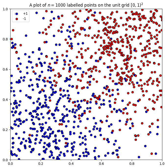
For our hypothesis class, we'll slice up the unit square into
For example, if we chose
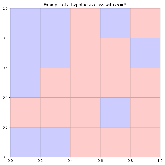
Note that each of the
where
Example of structural risk minimisation
Let's say we're trying to pick our model parameter
Because our data lies on the unit square, the random variables we used inside Hoeffding will be bounded by
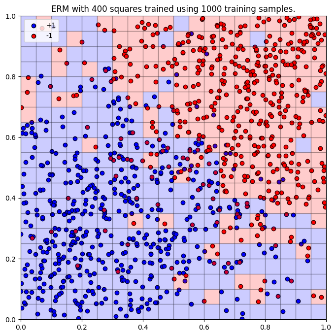
Why is this useful? Let's consider different examples with
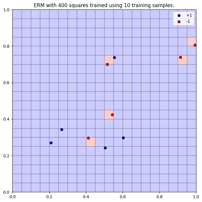
- If we had very little training data, say
, and we picked a very expressive model class, perhaps , then the -term in our 95% confidence bound evaluates to , meaning the risk of miscalculation is ludicrously high! Therefore, when applied to unseen data, this ERM will perform very poorly, only classifying the blue points correctly (without data, the ERM sets the square to blue as default).
- Equally, if we have access to lots of training data, say
, but retain model expressivity at , then the -term evaluates to , meaning that we still can't be confident that every possible ERM will perform well on unseen data. We're actually slightly overfitting with a 19% accuracy on 10,000 unseen data points.
If we consider the
Therefore, to improve our 95% confidence bound, we should aim for as small an
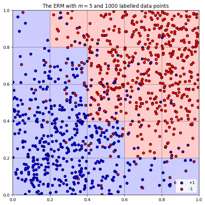
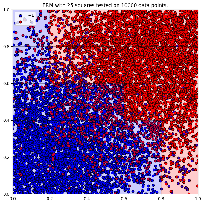
- Setting
, our -term further reduces to meaning we've structurally reduced the risk the furtherest out of the given examples. After computing an ERM on the training data points, we see that . Testing this ERM on 10,000 data points shows this is our best model yet with a 14% accuracy rate, pictured below:
While far from current practice, this toy example helps to elucidate the basic theory of generalisation in the case of binary classification with finite dimensional hypothesis classes.
Infinite Dimensional Hypothesis Classes
Now, we want to consider the trickier case where
Instead of studying the error directly, we'll consider the expected error, so applying an expectation to our previous bound, we want to study the following:
I.e. we want to bound
Rademacher Complexity
For notational ease, we'll bind our data together into
So, using this notation, we can unpick our definitions of risk and write
We're trying to formulate some notion of how complicated our hypothesis class is. We'll ask, 'on the
This intuition leads us to the Rademacher complexity as follows: if
- Call
. This is a collection of vectors in giving the behaviours of on the data . - The empirical Rademacher complexity is defined to be
- The
are Rademacher random variables, i.e. . This measures how close your classifier on your dataset is to random labels . E.g. if this is zero, then the model class is not particularly expressive, if this is 1 then the model class can achieve every possible labelling on data points. - Taking
to be random, you can view the empirical Rademacher complexity to be conditioned on the , so taking the expectation over , the Rademacher complexity is defined as
This post is quite long enough, so I'll defer to other resources that build intuition for the Rademacher complexity.
For our purposes, we want to use this concept to control the estimation error
So, we would like to estimate the RHS.
Connecting the Estimation Error to the Rademacher Complexity
To make this estimate, the key idea is to exploit the following symmetry.
- A random variable
is symmetric if and have the same distribution. - If
is a symmetric random variable and is a Rademacher random variable independent of , then and have the same distribution.
Result
Taking copies of random variables and bounding carefully yields the following result
where INSERT LINK TO ANNEX HERE
Connection to Estimation Error
So overall, we can put these bounds together to see that the estimation error is controlled by the Rademacher complexity:
Therefore, the problem of bounding the estimation error has been reduced to bounding the Rademacher complexity. How can we do this?
Connecting Rademacher Complexity to the Hypothesis Class
To gain an understanding of the expressivity of our function class
On fixed input data
If we unpick what's going on inside the Rademacher complexity term found above
We'll require some more tools from High-Dimensional Probability. Particularly, sub-gaussian random variables, which are simply random variables with tails that that decay like the gaussian/normal distribution. There are many equivalent definitions, but the most intuitive says that a random variable
Think 'strong tail decays' and see the annex for details. Using some key facts about these objects, we can argue as follows:
- The Rademacher random variables,
are sub-gaussian. LINK TO ANNEX - Sums of sub-gaussians are sub-gaussian (proof is definition pushing)
- Therefore, we have an expectation of a supremum over a finite set. If we pull out a probability textbook, there's a known result we can apply.
Fact: (proof in annex LINK TO ANNEX ) If
Application: If we let
Combining with our previous work, we now have a bound on the estimation error!
However, if we consider limits as
Vapnik-Chernovenkis (VC) dimension
First, we should ask, 'what is the worst case scenario?' We're in the case of binary classification. So with
Let
- We say
shatters data if . This means that every possible labelling is achieved on . - For this hypothesis class, we can define
to be the growth function or shattering coefficient. This measures the maximum number of behaviours of your hypothesis class on data points. As increases, the hypothesis class can express more and more behaviour until it reaches some cap based on the expressivity of . - The VC dimension of
is
- This measures largest number of data points where the hypothesis class
can fully shatter the dataset .
Example finding the VC dimension of a Hypothesis class
For example, if the hypothesis class consisted of half-open indicators on the real line
with
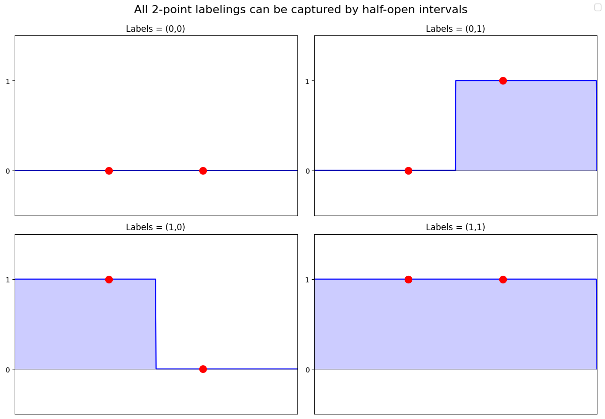
However
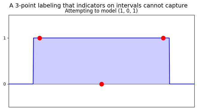
Thinking about general data
Sauer-Shalah Lemma
This example generalises! Here, I'll quote the most relevant formulation of the Sauer-Shelah lemma for our purpose: if
Hence, counting the behaviours of our hypothesis class on data
So in the case of binary classification, we have a method to measure the complexity of infinite dimensional hypothesis classes. Moreover, we can guarantee that the expected estimation error will tend to zero as the size of our training data tends to infinity. Neat!
While these bounds are too loose to be of real value in-practice, hopefully, this trip towards bounds of the expected risk during binary classification has been valuable. We've picked up some pretty mathematical tools which formalise some core concepts in modern ML.
Annex
A note on loss functions
In real world models, particularly during reinforcement learning, the design of loss functions is absolutely critical to ensure model safety. Lots of current research explores how different users of a model may have different metrics that they'd want to optimise for.
Linear Regression
Our goal is to find the
If we have a squint, this is just fancy Pythagoras! We're very close to our definition of the euclidian distance in
to be matrix with rows of length , then the matrix-vector product , gives us a vector of length . - Package up our
points into the vector
Putting this together, we can write this minimisation problem purely in terms of the norm! We want to minimise the distance:
This is a lovely least squares problem if we further package up our unknowns
Writing this out in a more friendly format, we have a neat relationship between the euclidian norm, the dot product and taking transposes, namely: if
Remember, this is a function of
So how do we go about differentiating this to find our ERM? Thinking about definitions, from school, we know that in 1d if we have some
As an illustrative example, if
In higher dimensions, we can use the same intuition, but need to be careful of the limit: now
We saw that the derivative of our function
In general, a function
Noting that we can take norms to deal with the 'dividing by a vector problem'. If this limit exists, then we can call the linear map
I'll skip over the formal epsilons and deltas and apply this definition in our calculation. What is the linear approximation to our function? We'll break it down into two parts:
For the harder part, we can use the definition and the same transpose trick as last time,
We can clearly inspect the term linear in
Putting this derivative to work and using the fact that our minimal solution will be achieved when the derivative is zero,
Which we can rearrange to get
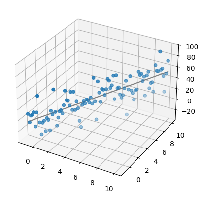
Neat! We can demo this was some basic toy data in Python. For
Tools from High-Dimensional Probability
Symmetrisation Argument
See the proof of theorem seven in Shah's MML lecture notes.
Rademacher Random Variables are sub-gaussian
Easy practice calculation here. Neatly our Rademacher random variables
Maximum of mean-zero sub-gaussians
Jensen's inequality says that for a random variable
Applying in our context with
Taking logs and optimising over LINK TO RESULT IN TEXT.
References
General
- Sharan, V. (n.d.). Rademacher calculation [PDF]. Available here. [Accessed 23 June 2025].
- Nakkiran, P., Kaplun, G., Bansal, Y., Yang, T., Barak, B. and Sutskever, I., 2019. A modern take on the bias-variance tradeoff in neural networks. arXiv preprint arXiv:1810.08591. Available here [Accessed 23 June 2025].
- Vershynin, R. (2018). High-Dimensional Probability: An Introduction with Applications in Data Science. Cambridge: Cambridge University Press. Available here [Accessed 23 June 2025].
- Stanford University, 2020. CS229M - Lecture 5: Rademacher complexity, empirical Rademacher complexity [video]. Available here [Accessed 23 June 2025].
- Lotz, M. (n.d.). Mathematics of Machine Learning. Available here [Accessed 23 June 2025].
- Shah, R. D. (n.d.). Machine Learning Lecture Notes [PDF]. University of Cambridge. Available here [Accessed 23 June 2025].
Personal
- Summary of Clarice Poon’s 2024 Mathematics of Machine Learning Lecture Notes. [online] Available here
- Summary of Mario Micallef’s 2023 Multivariable Calculus Lecture Notes. [online] Available here
- Summary of Stefan Adams’s 2024 High Dimensional Probability Lecture Notes. [online] Available here
- Summary of Krys Latuszynski’s 2023 Introduction to Mathematical Statistics Lecture Notes. [online] Available here